Tutorial on distribution approximation and posterior estimation
This notebook is an exercise in distribution approximation using Normalizing flows as implemented in the pyro library. The conditional Normalizing flow is also implemented using the zuko library (which is used in the AMPLFI library). The second half of the exercise shows the use case of posterior estimation using ML4GW tools.
Libraries needed for the notebook are
ml4gw==0.7.8pyro-pplzukolightningscikit-learn
# uncomment to install these dependencies
# ! pip install ml4gw==0.7.8 scikit-learn lightning pyro-ppl zuko
from typing import Callable, List

import h5py
import matplotlib.pyplot as plt
import numpy as np

from sklearn import datasets
from tqdm import tqdm

import torch
from torch import optim
from torch.distributions import Normal, TransformedDistribution

from pyro.nn import AutoRegressiveNN
from pyro.distributions.transforms import AffineAutoregressive

import zuko
torch.manual_seed(1)
# Check if GPU is available
device = torch.device("cuda" if torch.cuda.is_available() else "cpu")
print(f"Using device: {device}")
Using device: cuda
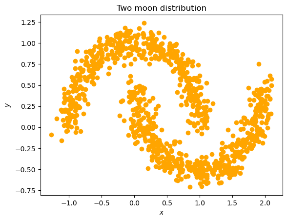
samples, labels = datasets.make_moons(n_samples=1000, noise=0.1)
Approximating the two-moon distribution
plt.scatter(samples.T[0], samples.T[1], color="orange")
plt.title("Two moon distribution")
plt.xlabel("$x$")
plt.ylabel("$y$")
Text(0, 0.5, '$y$')
samples = torch.from_numpy(samples).to(dtype=torch.float32, device=device)
Normalizing flow using Autoregressive Transforms
The normalizing flow we implement below has affine autoregressive transforms. Most of the constructs are available in the pyro API.
input_dim = 2  # data dimension
hidden_dims = [50*input_dim, 50*input_dim, 50*input_dim]

base_dist = Normal(
    torch.zeros(input_dim, device=device),
    torch.ones(input_dim, device=device)
)

arn = AutoRegressiveNN(
    input_dim,
    hidden_dims,
    param_dims=[1, 1]
).to(device)
# two dimensional input -> mu and sigma
with torch.no_grad():
    print(arn(torch.ones(1, 2, device=device)))
(tensor([[0.0149, 0.0908]], device='cuda:0'), tensor([[-0.0225, -0.0576]], device='cuda:0'))
transform = AffineAutoregressive(arn).to(device) # the "affine" part implies the linear relation between hidden dimensions
# the flow implementation is torch transformed distribution
flow_dist = TransformedDistribution(base_dist, [transform])
The flow_dist is the normalizing flow: It is a distribution which can be evaluated, and sampled from.
flow_dist.sample([10]) # -> 10 samples
tensor([[-0.3092,  2.6174],
        [-0.0878, -0.7060],
        [ 0.3213, -0.1771],
        [-1.4481,  2.3316],
        [ 0.0378, -2.5415],
        [-0.3469,  0.7560],
        [-1.3134, -0.0269],
        [-0.8357, -1.3689],
        [-0.4421,  0.1139],
        [-1.5013, -0.7086]], device='cuda:0')
# or evaluate the density
example_points = torch.tensor(
    [
        [0., 0.],
        [0., 1.],
        [1., 0.],
        [1., 1.],
    ],
    device=device
)
with torch.no_grad():
    sample_log_prob = flow_dist.log_prob(example_points)
for sample, log_prob in zip(example_points, sample_log_prob):
    print(f"log p({sample}) = {log_prob:.3e}")
log p(tensor([0., 0.], device='cuda:0')) = -1.749e+00
log p(tensor([0., 1.], device='cuda:0')) = -2.220e+00
log p(tensor([1., 0.], device='cuda:0')) = -2.252e+00
log p(tensor([1., 1.], device='cuda:0')) = -2.728e+00
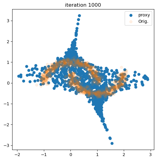
Now we learn this distribution
optimizer = optim.Adam(transform.parameters(), lr=1e-4)
from IPython.display import clear_output
from time import sleep

def live_plot(x_vals, y_vals, iteration, labels=None):
    """Auxiliary function to visualize the distribution"""
    clear_output(wait=True)
    sleep(1)
    fig, ax = plt.subplots(1, 1, figsize=(6, 6))
    ax.scatter(x_vals, y_vals, label='proxy')
    ax.scatter(samples.cpu().T[0], samples.cpu().T[1],
               alpha=0.1, label='Orig.', c=labels)
    ax.legend()
    ax.set_title('iteration {}'.format(iteration))
num_iter = 1000
for i in tqdm(range(num_iter)):
    optimizer.zero_grad()
    # take the original samples, and evaluate the likelihood.
    loss = -flow_dist.log_prob(samples).mean()
    loss.backward()
    optimizer.step()

    flow_dist.clear_cache()  # pyro modules cache values and derivatives for performance

    if (i + 1) % 100 == 0:
        with torch.no_grad():
            samples_flow = flow_dist.sample(torch.Size([1000,])).cpu().numpy()
        live_plot(samples_flow[:,0], samples_flow[:,1], i + 1)
        plt.show()
100%|███████████████████████████████████████████████████████████████████████████████████████████████████████████| 1000/1000 [00:14<00:00, 68.87it/s]
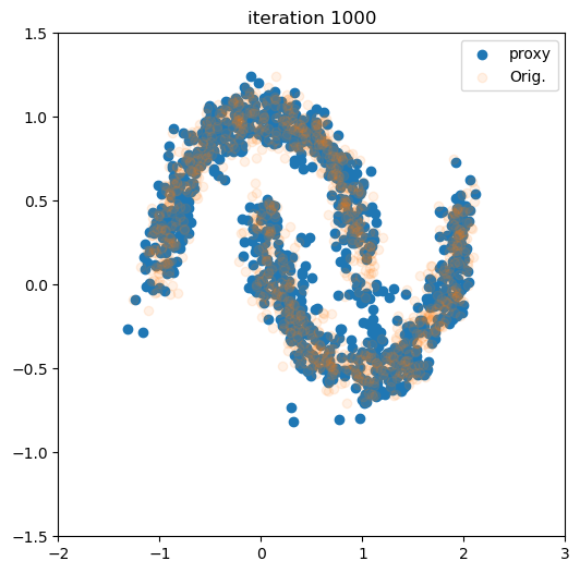
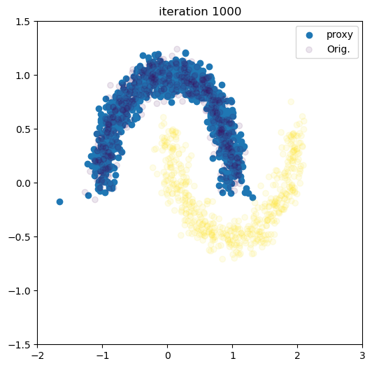
Compose several transforms
In the previous case we just had a single transform. Now we compose several of those and repeat
transforms = [
    AffineAutoregressive(
        AutoRegressiveNN(
            input_dim, hidden_dims,
            param_dims=[1, 1]
        ).to(device)
    ) for _ in range(10)
]

flow_dist = TransformedDistribution(base_dist, transforms)
trainable_parameters = []

for t in transforms:
    trainable_parameters.extend(list(t.parameters()))
optimizer = optim.Adam(trainable_parameters, lr=1e-4)
num_iter = 1000
for i in tqdm(range(num_iter)):

    optimizer.zero_grad()
    loss = -flow_dist.log_prob(samples).mean()
    loss.backward()
    optimizer.step()
    flow_dist.clear_cache()

    if (i + 1) % 100 == 0:
        with torch.no_grad():
            samples_flow = flow_dist.sample(
                torch.Size([1000,])
            ).cpu().numpy()

        live_plot(samples_flow[:,0], samples_flow[:,1], i + 1)
        plt.xlim((-2.0, 3.0))
        plt.ylim((-1.5, 1.5))
        plt.show()
100%|███████████████████████████████████████████████████████████████████████████████████████████████████████████| 1000/1000 [00:36<00:00, 27.37it/s]
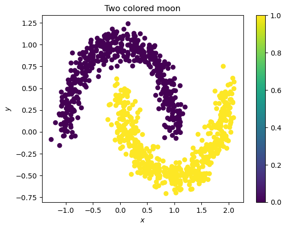
Condition and sample from each mode
plt.scatter(samples.cpu().T[0], samples.cpu().T[1], c=labels)
plt.title("Two colored moon")
plt.xlabel("$x$")
plt.ylabel("$y$")
plt.colorbar()
<matplotlib.colorbar.Colorbar at 0x7f705095b3d0>
labels = torch.from_numpy(labels).to(
    dtype=torch.float32,
    device=device
).reshape(samples.shape[0], 1)
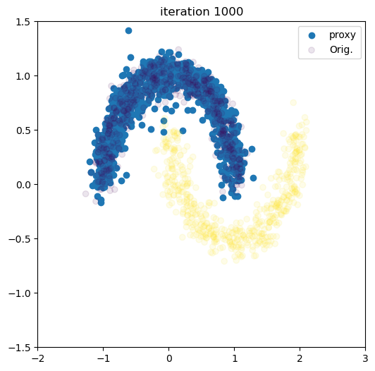
Conditional distribution
Let’s learn the conditional approximator based on the color
from pyro.distributions import ConditionalTransformedDistribution
from pyro.distributions.conditional import ConditionalComposeTransformModule
from pyro.nn.auto_reg_nn import ConditionalAutoRegressiveNN
from pyro.distributions.transforms import ConditionalAffineAutoregressive
condition_dim = 1 # the color is either 0 or 1
arn = ConditionalAutoRegressiveNN(
    input_dim,
    condition_dim,
    hidden_dims,
    param_dims=[1, 1]
).to(device)
with torch.no_grad():
    print(
        arn(
            torch.ones(5, 2, device=device),
            # need to supply additional context
            context=torch.ones(5, 1, device=device)
        )
    )
(tensor([[-0.1096, -0.0174],
        [-0.1096, -0.0174],
        [-0.1096, -0.0174],
        [-0.1096, -0.0174],
        [-0.1096, -0.0174]], device='cuda:0'), tensor([[-0.0531,  0.0315],
        [-0.0531,  0.0315],
        [-0.0531,  0.0315],
        [-0.0531,  0.0315],
        [-0.0531,  0.0315]], device='cuda:0'))
transforms = [
    ConditionalAffineAutoregressive(
        ConditionalAutoRegressiveNN(
            input_dim, condition_dim, hidden_dims,
            param_dims=[1, 1]
        ).to(device)
    ).to(device) for _ in range(5)
]
conditional_flow_dist = ConditionalTransformedDistribution(base_dist, transforms)
trainable_parameters = []
for t in transforms:
    trainable_parameters.extend(list(t.parameters()))

optimizer = optim.Adam(trainable_parameters, lr=1e-4)


num_iter = 1000
for i in tqdm(range(num_iter)):
    optimizer.zero_grad()
    loss = -conditional_flow_dist.condition(labels).log_prob(samples).mean()
    loss.backward()
    optimizer.step()
    conditional_flow_dist.clear_cache()

    if (i + 1) % 100 == 0:
        inference_label = ((i + 1) // 100) % 2  # alternate between modes
        with torch.no_grad():
            samples_one = conditional_flow_dist.condition(
                torch.tensor([inference_label,]).to(dtype=torch.float32, device=device)
            ).sample(torch.Size([1000,])).cpu().numpy()

        live_plot(samples_one[:,0], samples_one[:,1], i + 1, labels=labels.cpu())
        plt.xlim((-2.0, 3.0))
        plt.ylim((-1.5, 1.5))
        plt.show()
100%|███████████████████████████████████████████████████████████████████████████████████████████████████████████| 1000/1000 [00:24<00:00, 40.15it/s]
Conditional Normalizing Flow using zuko library
# defining the flow model using zuko's NSF flow - Neural Spline Flow

flow = zuko.flows.NSF(
    features=input_dim, # same as before which is 2
    context=condition_dim, # conditoning on just 1 context
    transforms=5, # number of transform layers, can be imported from zuko.flows.autoregressive or zuko.lazy
    hidden_features=hidden_dims, # same as before [100, 100, 100]
).to(device)
# testing the flow
with torch.no_grad():
    dist = flow(torch.ones(5, 1, device=device))
    print(dist.log_prob(torch.ones(5, 2, device=device)))
tensor([-2.9751, -2.9751, -2.9751, -2.9751, -2.9751], device='cuda:0')
optimizer = optim.Adam(flow.parameters(), lr=1e-4)

num_iter = 1000
for i in tqdm(range(num_iter)):
    optimizer.zero_grad()
    loss = -flow(labels).log_prob(samples)
    loss = loss.mean()
    loss.backward()
    optimizer.step()

    if (i + 1) % 100 == 0:
        inference_label = ((i + 1) // 100) % 2  # alternate between modes
        with torch.no_grad():
            samples_one = flow(
                torch.tensor([inference_label,]).to(dtype=torch.float32, device=device)
            ).sample(torch.Size([1000,])).cpu().numpy()

        live_plot(samples_one[:,0], samples_one[:,1], i + 1, labels=labels.cpu())
        plt.xlim((-2.0, 3.0))
        plt.ylim((-1.5, 1.5))
        plt.show()
100%|███████████████████████████████████████████████████████████████████████████████████████████████████████████| 1000/1000 [00:31<00:00, 31.78it/s]
Posterior estimation of gravitational-wave events
Get background data from LIGO detectors
We will download some data from Sept 15, 2015, the day after the detection of GW150914
from gwpy.timeseries import TimeSeries, TimeSeriesDict
from pathlib import Path

# Point this to whatever directory you want to house
# all of the data products this notebook creates
data_dir = Path("/tmp/data")

# And this to the directory where you want to download the data
background_dir = data_dir / "background_data"
background_dir.mkdir(parents=True, exist_ok=True)

# This is a 10000s segment on Sept 15, 2015, the day after
# GW150914 was detected
segments = [
    (1126310417, 1126320417),
]
ifos = ["H1", "L1"]  # Hanford and Livingston
sample_rate = 2048  # Hz

for (start, end) in segments:
    # Download the data from GWOSC. This will take a few minutes.
    duration = end - start
    fname = background_dir / f"background-{start}-{duration}.hdf5"
    if fname.exists():
        continue

    ts_dict = TimeSeriesDict()
    for ifo in ifos:
        ts_dict[ifo] = TimeSeries.fetch_open_data(ifo, start, end, cache=True)
    ts_dict = ts_dict.resample(sample_rate)
    ts_dict.write(fname, format="hdf5")
/u/bgupta1/.conda/envs/mlgw/lib/python3.10/site-packages/gwpy/time/__init__.py:36: UserWarning: Wswiglal-redir-stdio:

SWIGLAL standard output/error redirection is enabled in IPython.
This may lead to performance penalties. To disable locally, use:

with lal.no_swig_redirect_standard_output_error():
    ...

To disable globally, use:

lal.swig_redirect_standard_output_error(False)

Note however that this will likely lead to error messages from
LAL functions being either misdirected or lost when called from
Jupyter notebooks.

To suppress this warning, use:

import warnings
warnings.filterwarnings("ignore", "Wswiglal-redir-stdio")
import lal

  from lal import LIGOTimeGPS
Create simulations using ML4GW tools
from torch.distributions import Uniform

# ml4gw components
from ml4gw.waveforms import IMRPhenomD
from ml4gw.waveforms.generator import TimeDomainCBCWaveformGenerator
from ml4gw.waveforms.conversion import chirp_mass_and_mass_ratio_to_components

from ml4gw.gw import compute_observed_strain, get_ifo_geometry

from ml4gw.transforms import Whiten, SpectralDensity
from ml4gw.distributions import PowerLaw, Sine, Cosine
We will use InMemoryDataset for dataloading. This can send the entire background to the GPU memory before training commences, and generates waveforms on-the-fly.
This is useful for prototyping with small background stretches that is not too large to fit in device memory.
from ml4gw.dataloading import InMemoryDataset
# define priors to generate waveforms
prior_dict = {
    "chirp_mass": Uniform(25, 35),
    "mass_ratio": Uniform(0.125, 0.999),
    "chi1": Uniform(-0.999, 0.999),
    "chi2": Uniform(-0.999, 0.999),
    "distance": PowerLaw(300, 700, 2.0),
    "phic": Uniform(0, 2*torch.pi),
    "inclination": Sine()
}
We will infer only on a subset of parameters for this exercise
# define inference parameters for posterior estimation
inference_params = {k:prior_dict[k] for k in ['chirp_mass', 'distance']}
The InMemoryDataset is an IterableDataset that lazily loads batches from the background that is in device memory. We create a derived class that adds the capacity to do injections on top of lazily loaded batches.
The main method below is inject. This yields a new background batch, dynamically estimates the PSD, generates and injects a batch of waveforms, and whitens it with the estimated PSD, all using ml4gw tools.
class InMemoryInjectionDataset(InMemoryDataset):
    def __init__(
        self,
        X,
        ifos: List[str] = ["H1", "L1"],
        kernel_length: int = 4.0,
        # PSD/whitening args
        fduration: float = 2,
        psd_length: float = 16,
        sample_rate: float = 2048,
        fftlength: float = 2,
        highpass: float = 32,
        # Dataloading args
        batch_size: int = 10,
        batches_per_epoch: int = 100,
        approximant = IMRPhenomD,
        prior_dict = prior_dict,
        f_min: float = 20,
        f_max: float = None,
        f_ref: float = 20,
        device: torch.device = device,
    ):
        self.kernel_size = int(kernel_length * sample_rate)
        self.sample_rate = sample_rate
        self.fduration = fduration
        self.window_size = self.kernel_size + int(fduration * sample_rate)
        self.psd_size = int(psd_length * sample_rate)
        self.batch_size = batch_size
        self.batches_per_epoch = batches_per_epoch
        self.device = device
        super().__init__(
            X,
            self.window_size + self.psd_size,
            None,
            self.batch_size,
            stride=1,
            batches_per_epoch=self.batches_per_epoch,
            coincident=False,
            shuffle=True,
            device=self.device,
        )
        self.ifos = ifos
        # real-time transformations defined with torch Modules
        self.spectral_density = SpectralDensity(
            sample_rate, fftlength, average="median", fast=False
        ).to(self.device)
        self.whitener = Whiten(
            fduration, sample_rate, highpass=highpass
        ).to(self.device)
        # define some sky parameter distributions
        self.prior_dict = prior_dict
        torch_pi = torch.as_tensor(torch.pi, device=self.device)
        self.dec = Cosine(-torch_pi / 2, torch_pi / 2)
        self.psi = torch.distributions.Uniform(0, torch_pi)
        self.phi = torch.distributions.Uniform(
            -torch_pi, torch_pi
        )  # relative RAs of detector and source
        self.approx = approximant().to(self.device)
        self.waveform_generator = TimeDomainCBCWaveformGenerator(
            approximant=self.approx,
            sample_rate=sample_rate,
            duration=kernel_length + fduration,
            f_min=f_min,
            f_ref=f_ref,
            right_pad=0.5,  # this means the merger is 0.5 seconds from the end
        ).to(self.device)
        self.detector_tensors, self.detector_vertices = get_ifo_geometry(*ifos)
        self.detector_tensors = self.detector_tensors.to(self.device)
        self.detector_vertices = self.detector_vertices.to(self.device)

    def project_waveforms(
        self, hc: torch.Tensor, hp: torch.Tensor
    ) -> torch.Tensor:
        # sample sky parameters
        N = len(hc)
        dec = self.dec.sample((N,)).to(hc)
        psi = self.psi.sample((N,)).to(hc)
        phi = self.phi.sample((N,)).to(hc)

        proj_params = {
            "dec": dec,
            "psi": psi,
            "phi": phi,
        }
        # project to interferometer response
        return compute_observed_strain(
            dec=dec,
            psi=psi,
            phi=phi,
            detector_tensors=self.detector_tensors,
            detector_vertices=self.detector_vertices,
            sample_rate=self.sample_rate,
            cross=hc,
            plus=hp,
        ), proj_params

    def generate_waveforms(self, batch_size: int) -> tuple[torch.Tensor, ...]:
        params = {
            k: v.sample((batch_size,)).to(self.device)
            for k, v in self.prior_dict.items()
        }
        # attach component masses if not present
        if "mass_1" not in params:
            params["mass_1"], params["mass_2"] = chirp_mass_and_mass_ratio_to_components(
                params["chirp_mass"], params["mass_ratio"]
            )
        if "s1z" not in params:
            params["s1z"], params["s2z"] = params["chi1"], params["chi2"]
        hc, hp = self.waveform_generator(**params)
        return hc, hp, params

    def inject(self, X: torch.Tensor) -> tuple[torch.Tensor, torch.Tensor]:
        # break off "background" from target kernel and compute its PSD
        # (in double precision since our scale is so small)
        background, X = torch.split(
            X, [self.psd_size, self.window_size], dim=-1
        )
        psd = self.spectral_density(background.double())

        # generate polarizations
        hc, hp, params = self.generate_waveforms(self.batch_size)

        # project
        responses, proj_params = self.project_waveforms(hc, hp)

        # include sky params in returned params
        params.update(proj_params)

        # inject waveform into background and whiten
        X += responses.float()
        X = self.whitener(X, psd)

        return X, params

    def __iter__(self):
        for X in super().__iter__():
            X, params = self.inject(X)
            yield X, params
Now create a Lightning datamodule using the above dataset.
import pytorch_lightning as pl
/u/bgupta1/.conda/envs/mlgw/lib/python3.10/site-packages/torchmetrics/utilities/imports.py:22: UserWarning: pkg_resources is deprecated as an API. See https://setuptools.pypa.io/en/latest/pkg_resources.html. The pkg_resources package is slated for removal as early as 2025-11-30. Refrain from using this package or pin to Setuptools<81.
  from pkg_resources import DistributionNotFound, get_distribution
class ML4GWInferenceDatamodule(pl.LightningDataModule):
    def __init__(
        self,
        background_file,
        ifos: List[str] = ["H1", "L1"],
        kernel_length: int = 4.0,
        # PSD/whitening args
        fduration: float = 2,
        psd_length: float = 16,
        sample_rate: float = 2048,
        fftlength: float = 2,
        highpass: float = 32,
        # Dataloading args
        batch_size: int = 10,
        batches_per_epoch: int = 100,
        approximant = IMRPhenomD,
        prior_dict = prior_dict,
        inference_params = inference_params,
        valid_frac: float = 0.2,
        f_min: float = 20,
        f_max: float = None,
        f_ref: float = 20,
    ):
        super().__init__()
        self.save_hyperparameters(
            ignore=[
                "background_file",
                "ifos",
                "approximant",
                "prior_dict",
                "inference_params"
            ]
        )
        self.background_file = background_file
        self.ifos = ifos
        self.approximant = approximant
        self.prior_dict = prior_dict
        self.inference_params = inference_params

    def setup(self, stage: str) -> None:
        if stage == 'fit' or stage == 'validate':
            # load background data
            background = []
            with h5py.File(self.background_file) as f:
                for ifo in self.ifos:
                    hoft = f[ifo][:]
                    background.append(hoft)
            background = torch.from_numpy(np.stack(background))
            # background, valid_background = split(
            #     background, 1 - self.hparams.valid_frac, 1)
            valid_background_size = int(self.hparams.valid_frac * background.shape[-1])
            background, valid_background = torch.split(
                background,
                [
                    background.shape[-1] - valid_background_size,
                    valid_background_size
                ],
                dim=-1
            )
            device = self.trainer.model.device if self.trainer else "cpu"
            common_kwargs = dict(
                ifos=self.ifos,
                kernel_length=self.hparams.kernel_length,
                fduration=self.hparams.fduration,
                psd_length=self.hparams.psd_length,
                sample_rate=self.hparams.sample_rate,
                fftlength=self.hparams.fftlength,
                highpass=self.hparams.highpass,
                batch_size=self.hparams.batch_size,
                batches_per_epoch=self.hparams.batches_per_epoch,
                approximant=self.approximant,
                prior_dict=self.prior_dict,
                f_min=self.hparams.f_min,
                f_max=self.hparams.f_max,
                f_ref=self.hparams.f_ref,
                device=device,
            )
            self.training_dataset = InMemoryInjectionDataset(
                background,
                **common_kwargs
            )
            self.validation_dataset = InMemoryInjectionDataset(
                valid_background,
                **common_kwargs
            )

    def train_dataloader(self):
        return self.training_dataset

    def val_dataloader(self):
        return self.validation_dataset
# example usage of the datamodule
datamodule = ML4GWInferenceDatamodule(background_dir / "background-1126310417-10000.hdf5")
datamodule.setup('validate')
for X_inj, param in datamodule.val_dataloader():
    break
print(X_inj.shape)
print(param['chirp_mass'])
torch.Size([10, 2, 8192])
tensor([30.0488, 28.2032, 30.3778, 25.4208, 29.7266, 29.3884, 29.9440, 28.1072,
        34.8015, 29.8784])
Now we build the Normalizing flow as a LightningModule
The module has a learnable architecture which is used to summarize the strain data. The normalizing flow learns the distribution of the inference parameters given this data summary.
class ML4GWInferenceModel(pl.LightningModule):
    """A LFI model using ML4GW tools"""
    def __init__(
        self,
        architecture: torch.nn.Module,
        inference_params: List[str] = inference_params,
        num_transforms: int = 20,
        num_blocks: int = 5,
        hidden_features: int = 250,
        context_dim: int = 32,
        learning_rate: float = 0.001,
        activation: Callable = torch.nn.Tanh,
    ) -> None:
        super().__init__()
        self.save_hyperparameters(
            ignore=["architecture",]
        )
        self.nn = architecture
        # build the normalizing flow
        self.param_dim = len(inference_params)
        self.build_flow()

    def embedding_net(self, X):
        return self.nn(X)

    def training_step(self, batch, _):
        strain, param_dict = batch
        params = []
        for _ in self.hparams.inference_params.keys():
            params.append(param_dict[_])
        params = torch.stack(params, dim=1)
        loss = -self.log_prob(params, context=strain).mean()
        self.log(
            "train_loss", loss, on_step=True, prog_bar=True, sync_dist=False
        )
        return loss

    def validation_step(self, batch, _):
        strain, param_dict = batch
        params = []
        for _ in self.hparams.inference_params.keys():
            params.append(param_dict[_])
        params = torch.stack(params, dim=1)
        loss = -self.log_prob(params, context=strain).mean()
        self.log(
            "valid_loss", loss, on_epoch=True, prog_bar=True, sync_dist=True
        )
        return loss

    def configure_optimizers(self):
        optimizer = torch.optim.AdamW(self.parameters(), self.hparams.learning_rate)
        scheduler = torch.optim.lr_scheduler.OneCycleLR(
            optimizer,
            self.hparams.learning_rate,
            pct_start=0.1,
            total_steps=self.trainer.estimated_stepping_batches,
        )
        scheduler_config = dict(scheduler=scheduler, interval="step")
        return dict(optimizer=optimizer, lr_scheduler=scheduler_config)

    def configure_callbacks(self):
        chkpt = pl.callbacks.ModelCheckpoint(monitor="valid_loss", mode="min")
        return [chkpt]

    def transform_block(self):
        """Returns single autoregressive transform"""
        param_dim = len(self.hparams.inference_params)
        arn = ConditionalAutoRegressiveNN(
            param_dim,
            self.hparams.context_dim,
            self.hparams.num_blocks * [self.hparams.hidden_features],
            nonlinearity=self.hparams.activation(),
        )
        transform = ConditionalAffineAutoregressive(arn)
        return transform

    def flow(self):
        if not hasattr(self, "transforms"):
            raise RuntimeError("Flow is not built")
        return ConditionalTransformedDistribution(
            self.distribution(), self.transforms
        )

    def distribution(self):
        """Returns the base distribution for the flow"""
        return Normal(
            torch.zeros(self.param_dim, device=self.device),
            torch.ones(self.param_dim, device=self.device),
        )

    def build_flow(self):
        """Build the transform"""
        self.transforms = []
        for idx in range(self.hparams.num_transforms):
            _transform = self.transform_block()
            self.transforms.extend([_transform])
        self.transforms = ConditionalComposeTransformModule(self.transforms)

    def log_prob(self, x, context):
        """Wrapper `log_prob` from TransformedDistribution"""
        if not hasattr(self, "transforms"):
            raise RuntimeError("Flow is not built")
        embedded_context = self.embedding_net(context)
        flow = self.flow()
        return flow.condition(embedded_context).log_prob(x)

    def sample(self, n, context):
        """Wrapper around sample from TransformedDistribution object"""
        if not hasattr(self, "transforms"):
            raise RuntimeError("Flow is not built")
        n = [n] if isinstance(n, int) else n
        embedded_context = self.embedding_net(context)
        flow = self.flow()
        return flow.condition(embedded_context).sample(n)
from ml4gw.nn.resnet import ResNet1D
# we use a ResNet1D as the embedding network
architecture = ResNet1D(
    in_channels=2,
    layers=[5, 5],
    classes=32,
    kernel_size=5,
)
log_dir = "/tmp/pl-logs"

logger = pl.loggers.CSVLogger(log_dir, name="ml4gw-lfi-expt")

# create a fresh instance of the model
model = ML4GWInferenceModel(
    architecture=architecture,
)
datamodule = ML4GWInferenceDatamodule(
    background_dir / "background-1126310417-10000.hdf5",
    batch_size=500  # adjust based on your device memory
)
# invoke trainer
trainer = pl.Trainer(
    max_epochs=30,
    check_val_every_n_epoch=5,
    precision="16-mixed",
    log_every_n_steps=20,
    logger=logger,
    accelerator="auto",
)
trainer.fit(model, datamodule=datamodule)
/u/bgupta1/.conda/envs/mlgw/lib/python3.10/site-packages/lightning_fabric/plugins/environments/slurm.py:204: The `srun` command is available on your system but is not used. HINT: If your intention is to run Lightning on SLURM, prepend your python command with `srun` like so: srun python /u/bgupta1/.conda/envs/mlgw/lib/python3.10/site-pack ...
Using 16bit Automatic Mixed Precision (AMP)
💡 Tip: For seamless cloud uploads and versioning, try installing [litmodels](https://pypi.org/project/litmodels/) to enable LitModelCheckpoint, which syncs automatically with the Lightning model registry.
GPU available: True (cuda), used: True
TPU available: False, using: 0 TPU cores
HPU available: False, using: 0 HPUs
The following callbacks returned in `LightningModule.configure_callbacks` will override existing callbacks passed to Trainer: ModelCheckpoint
You are using a CUDA device ('NVIDIA A40') that has Tensor Cores. To properly utilize them, you should set `torch.set_float32_matmul_precision('medium' | 'high')` which will trade-off precision for performance. For more details, read https://pytorch.org/docs/stable/generated/torch.set_float32_matmul_precision.html#torch.set_float32_matmul_precision
LOCAL_RANK: 0 - CUDA_VISIBLE_DEVICES: [0]
Loading `train_dataloader` to estimate number of stepping batches.
/u/bgupta1/.conda/envs/mlgw/lib/python3.10/site-packages/pytorch_lightning/utilities/model_summary/model_summary.py:231: Precision 16-mixed is not supported by the model summary.  Estimated model size in MB will not be accurate. Using 32 bits instead.

  | Name       | Type                              | Params | Mode
-------------------------------------------------------------------------
0 | nn         | ResNet1D                          | 1.0 M  | train
1 | transforms | ConditionalComposeTransformModule | 5.2 M  | train
-------------------------------------------------------------------------
6.2 M     Trainable params
0         Non-trainable params
6.2 M     Total params
24.862    Total estimated model params size (MB)
274       Modules in train mode
0         Modules in eval mode
/u/bgupta1/.conda/envs/mlgw/lib/python3.10/site-packages/torch/optim/lr_scheduler.py:224: UserWarning: Detected call of `lr_scheduler.step()` before `optimizer.step()`. In PyTorch 1.1.0 and later, you should call them in the opposite order: `optimizer.step()` before `lr_scheduler.step()`.  Failure to do this will result in PyTorch skipping the first value of the learning rate schedule. See more details at https://pytorch.org/docs/stable/optim.html#how-to-adjust-learning-rate
  warnings.warn(
`Trainer.fit` stopped: `max_epochs=30` reached.
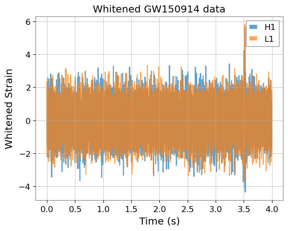
Test model against GW150914
We will download data around GW150914 and whiten it using ml4gw tools
model.eval()
ML4GWInferenceModel(
  (nn): ResNet1D(
    (conv1): Conv1d(2, 64, kernel_size=(7,), stride=(2,), padding=(3,), bias=False)
    (bn1): GroupNorm1D()
    (relu): ReLU(inplace=True)
    (maxpool): MaxPool1d(kernel_size=3, stride=2, padding=1, dilation=1, ceil_mode=False)
    (residual_layers): ModuleList(
      (0): Sequential(
        (0): BasicBlock(
          (conv1): Conv1d(64, 64, kernel_size=(5,), stride=(1,), padding=(2,), bias=False)
          (bn1): GroupNorm1D()
          (relu): ReLU(inplace=True)
          (conv2): Conv1d(64, 64, kernel_size=(5,), stride=(1,), padding=(2,), bias=False)
          (bn2): GroupNorm1D()
        )
        (1): BasicBlock(
          (conv1): Conv1d(64, 64, kernel_size=(5,), stride=(1,), padding=(2,), bias=False)
          (bn1): GroupNorm1D()
          (relu): ReLU(inplace=True)
          (conv2): Conv1d(64, 64, kernel_size=(5,), stride=(1,), padding=(2,), bias=False)
          (bn2): GroupNorm1D()
        )
        (2): BasicBlock(
          (conv1): Conv1d(64, 64, kernel_size=(5,), stride=(1,), padding=(2,), bias=False)
          (bn1): GroupNorm1D()
          (relu): ReLU(inplace=True)
          (conv2): Conv1d(64, 64, kernel_size=(5,), stride=(1,), padding=(2,), bias=False)
          (bn2): GroupNorm1D()
        )
        (3): BasicBlock(
          (conv1): Conv1d(64, 64, kernel_size=(5,), stride=(1,), padding=(2,), bias=False)
          (bn1): GroupNorm1D()
          (relu): ReLU(inplace=True)
          (conv2): Conv1d(64, 64, kernel_size=(5,), stride=(1,), padding=(2,), bias=False)
          (bn2): GroupNorm1D()
        )
        (4): BasicBlock(
          (conv1): Conv1d(64, 64, kernel_size=(5,), stride=(1,), padding=(2,), bias=False)
          (bn1): GroupNorm1D()
          (relu): ReLU(inplace=True)
          (conv2): Conv1d(64, 64, kernel_size=(5,), stride=(1,), padding=(2,), bias=False)
          (bn2): GroupNorm1D()
        )
      )
      (1): Sequential(
        (0): BasicBlock(
          (conv1): Conv1d(64, 128, kernel_size=(5,), stride=(2,), padding=(2,), bias=False)
          (bn1): GroupNorm1D()
          (relu): ReLU(inplace=True)
          (conv2): Conv1d(128, 128, kernel_size=(5,), stride=(1,), padding=(2,), bias=False)
          (bn2): GroupNorm1D()
          (downsample): Sequential(
            (0): Conv1d(64, 128, kernel_size=(1,), stride=(2,), bias=False)
            (1): GroupNorm1D()
          )
        )
        (1): BasicBlock(
          (conv1): Conv1d(128, 128, kernel_size=(5,), stride=(1,), padding=(2,), bias=False)
          (bn1): GroupNorm1D()
          (relu): ReLU(inplace=True)
          (conv2): Conv1d(128, 128, kernel_size=(5,), stride=(1,), padding=(2,), bias=False)
          (bn2): GroupNorm1D()
        )
        (2): BasicBlock(
          (conv1): Conv1d(128, 128, kernel_size=(5,), stride=(1,), padding=(2,), bias=False)
          (bn1): GroupNorm1D()
          (relu): ReLU(inplace=True)
          (conv2): Conv1d(128, 128, kernel_size=(5,), stride=(1,), padding=(2,), bias=False)
          (bn2): GroupNorm1D()
        )
        (3): BasicBlock(
          (conv1): Conv1d(128, 128, kernel_size=(5,), stride=(1,), padding=(2,), bias=False)
          (bn1): GroupNorm1D()
          (relu): ReLU(inplace=True)
          (conv2): Conv1d(128, 128, kernel_size=(5,), stride=(1,), padding=(2,), bias=False)
          (bn2): GroupNorm1D()
        )
        (4): BasicBlock(
          (conv1): Conv1d(128, 128, kernel_size=(5,), stride=(1,), padding=(2,), bias=False)
          (bn1): GroupNorm1D()
          (relu): ReLU(inplace=True)
          (conv2): Conv1d(128, 128, kernel_size=(5,), stride=(1,), padding=(2,), bias=False)
          (bn2): GroupNorm1D()
        )
      )
    )
    (avgpool): AdaptiveAvgPool1d(output_size=1)
    (fc): Linear(in_features=128, out_features=32, bias=True)
  )
  (transforms): ConditionalComposeTransformModule(
    (0-19): 20 x ConditionalAffineAutoregressive(
      (nn): ConditionalAutoRegressiveNN(
        (layers): ModuleList(
          (0): MaskedLinear(in_features=34, out_features=250, bias=True)
          (1-4): 4 x MaskedLinear(in_features=250, out_features=250, bias=True)
          (5): MaskedLinear(in_features=250, out_features=4, bias=True)
        )
        (f): Tanh()
      )
    )
  )
)
# Download and whiten GW150914 data
from gwpy.timeseries import TimeSeries

trigger_time = 1126259462.4
duration = 6
post_trigger_duration = 1.5  # whitening will trim 1s on each side
end_time = trigger_time + post_trigger_duration
start_time = end_time - duration

psd_duration = 4 * duration
psd_start_time = start_time - psd_duration
psd_end_time = start_time

data_ts = []
psd_data_ts = []
for det in ["H1", "L1"]:
    print("Downloading analysis data for ifo {}".format(det))
    data = TimeSeries.fetch_open_data(det, start_time, end_time)
    data = data.resample(sample_rate)
    data_ts.append(
        torch.from_numpy(data.value.copy()))
    print("Downloading psd data for ifo {}".format(det))
    psd_data = TimeSeries.fetch_open_data(det, psd_start_time, psd_end_time)
    psd_data = psd_data.resample(sample_rate)
    psd_data_ts.append(
        torch.from_numpy(psd_data.value.copy()))
Downloading analysis data for ifo H1
Downloading psd data for ifo H1
Downloading analysis data for ifo L1
Downloading psd data for ifo L1
fftlength = 2
fduration = 2

spectral_density = SpectralDensity(
    sample_rate=sample_rate,
    fftlength=fftlength,
    overlap=None,
    average="median",
)

whiten = Whiten(
    fduration=fduration,
    sample_rate=sample_rate,
    highpass=20
)

data_whitened = []
for data, psd_data in zip(data_ts, psd_data_ts):
    psd = spectral_density(psd_data)
    data_whitened.append(whiten(data, psd).squeeze())

data_whitened = torch.stack(data_whitened)
times = torch.linspace(0, duration - fduration, int(sample_rate * (duration - fduration)))
for d_whitened, det in zip(data_whitened, ['H1', 'L1']):
    plt.plot(times, d_whitened.cpu().numpy(), label=det, alpha=0.7)
plt.title("Whitened GW150914 data")
plt.legend()
plt.xlabel("Time (s)")
plt.ylabel("Whitened Strain")
Text(0, 0.5, 'Whitened Strain')
Sample from the flow, using the whitened data as context
samples = model.sample(n=10000, context=data_whitened.unsqueeze(0))
from corner import corner
figure = corner(
    samples.cpu().numpy(),
    labels=[
        r"$M_c$",
        r"$D_L$",
    ],
    quantiles=[0.1, 0.5, 0.9],
    show_titles=True,
    title_kwargs={"fontsize": 12},
)
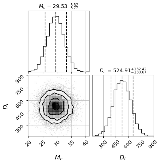
This is not the best constraining result since the flow needs to train for longer. For reference the results from GWTC-1 is \(M_c = 28.6^{+1.7}_{-1.5}\;M_{\odot}\) and \(D_L = 440^{+150}_{-170}\). But it is in the ballpark.
There are a few key improvements in the production models deployed in LIGO-Virgo-KAGRA fourth observing run, compared to this tutorial (see the AMPLFI methods and validation papers):
A multimodal embedding network involving both time and frequency-domain data views
Standard scaling the parameters before forward-modeling with the normalizing flow
Marginalizing over a time-of-arrival window using data augmentation and self-supervised learning